

When programming, we often hear the question, “What is the time complexity of this program?” But what is a program, really? If we think about it, every program or software is essentially a set of fixed operations. These operations, such as assignment (a = 2) or conditional checks (a < 0), require time to execute when the program runs.
In simple terms, time complexity measures how much time a program takes to solve a specific input.
We know that a problem can have multiple solutions. For example, if I can complete a task in 5 hours and you can do it in 1 hour, your method is more efficient than mine in terms of time. Similarly, in programming, when comparing multiple solutions, the one with better time complexity is considered more optimal.
However, we don’t measure the exact time in seconds; instead, we analyze the growth of time relative to the input size. This growth rate helps us differentiate between good and bad solutions. The question then becomes, how do we measure this complexity?
Measuring Time Complexity
One might think of running different solutions with the same input, timing their execution, and comparing the results. But this approach has several flaws:
- Machine Dependency: The runtime of a program depends on the machine it runs on. A slow algorithm on a powerful, modern computer might outperform a good algorithm on an older, less capable machine.
- Input Scalability: A program might perform well for small inputs (e.g., 100, 1,000, or 10,000), but fail miserably for larger inputs (e.g., 1 million).
Thus, manual testing isn’t efficient. Instead, we use asymptotic analysis to evaluate an algorithm’s performance as the input size changes.
Types of Time Complexity
Time complexity is often categorized into three scenarios:
- Best Case: Represented by Ω(n) (Omega notation), this measures the minimum time an algorithm takes for the best possible input. For example, finding the smallest number in a sorted array always takes constant time Ω(1)\text{Ω(1)}Ω(1). However, best-case complexity is rarely useful in real-life scenarios.
- Average Case: Represented by Θ(n) (Theta notation), this measures the average time taken over all possible inputs. While insightful, it’s also less commonly used in practice.
- Worst Case: Represented by O(n) (Big-O notation), this measures the maximum time an algorithm takes for the worst possible input. This is the most practical measure, as it defines the upper bound of the algorithm’s time requirement.
- in real life we are focused on this, when we are desinging a solution we need to think how our solution will perform in this worst case scenarios.
Example: Searching in an Array
Let’s say we need to search for a number in an array. The worst-case scenario would be:
- The number isn’t in the array.
- The number is at the last position, and we start searching from the beginning.
Here, we’d have to check every element, making the complexity O(n), where nnn is the size of the array.
For instance:
- If there are 100 numbers and it takes 1 second to check each, it would take 100 seconds.
- For 200 numbers, it would take 200 seconds.
This shows a linear relationship between input size and execution time.
Implications of Time Complexity
Knowing the time complexity helps us:
Choose Efficient Algorithms: If a program must complete within 120 seconds, and the input size is 100, we know we need a linear or better solution.
Optimize Solutions: If a program takes 500 seconds to search among 100 numbers, but we know a solution exists that can do it in 100 seconds, we realize there’s room for improvement.
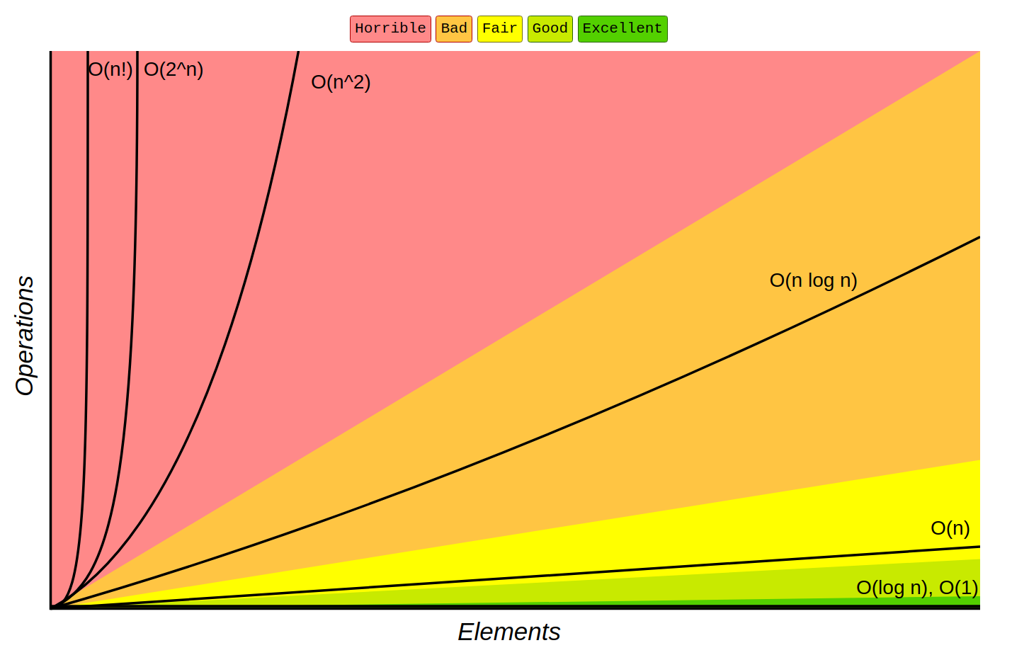
Big-O Complexity Cheat Sheet
The following chart provides an overview of common time complexities, ordered from best to worst:
| Complexity | Example Solution Type |
|---|---|
| O(1) | Constant Time |
| O(log n) | Logarithmic (e.g., Binary Search) |
| O(n) | Linear |
| O(n log n) | Linearithmic (e.g., Merge Sort) |
| O(n²) | Quadratic (e.g., Nested Loops) |
| O(n!) | Factorial (e.g., Permutations) |
For instance:
- With O(n) for 50 elements, the program performs 50 operations.
- A quadratic O(n2) solution will perform O(502)=2,500 operations.
- With O(n!), the program performs 50! operations—a staggering number you’ll likely need to Google!

In this chart, we can see that the best solution is one with constant time complexity, followed by logarithmic, then linear, and so on, with factorial being the worst. This graph represents the relationship between the number of elements and the number of operations.
By understanding time complexity, we can select or design algorithms that are both efficient and scalable.


